Recipe for russell et al figures 1, 2, 3a, 3b, 4, 5, 5g, 6a, 6b, 7, 7h, 7i, 8, 9a, 9b, 9c. Russell, J.L.,et al., 2018, J. Geophysical Research - Oceans, 123, 3120-3143, https://doi.org/10.1002/2017JC013461 Please read individual description in diagnostics section.
Diagnostic for russell et al figure 1. Plots Annual-mean zonal wind stress as polar contour map. Here, we are using tauuo. Figures in russell18jgr paper were made using tauuo, but tauu can also be used if tauuo file is not available. To use tauu variable in this recipe just uncomment variable 'tauu' and add dataset names in additional datasets of respective variable. If there are no dataset in a variable, entire variable section needs to be commented out.

Diagnostic for russell et al Figure 2. Plots The zonal and annual means of the zonal wind stress (N/m^2). Here, we are using tauuo, figures in russell18jgr paper were made using tauuo, but tauu can also be used if tauuo file is not available. To use tauu variable in this recipe just uncomment variable 'tauu' and add dataset names in additional datasets of respective variable. If there are no dataset in a variable, entire variable section needs to be commented out.

Diagnostic for russell et al figure 3b. Plots the latitudinal position of Subantarctic Front. Using definitions from Orsi et al (1995), the Subantarctic Front is defined here as the poleward location of the 4C(277.15K) isotherm at(closest to and less than) 400 m.

Diagnostic for russell et al figure 3b-2 (Polar fronts). Plots the latitudinal position of Polar Front. Using definitions from Orsi et al. (1995). The Polar Front is defined here as the poleward location of the 2C (275.15K) isotherm of the temperature minimum between 0 and 200 m (closest to and less than 200m).

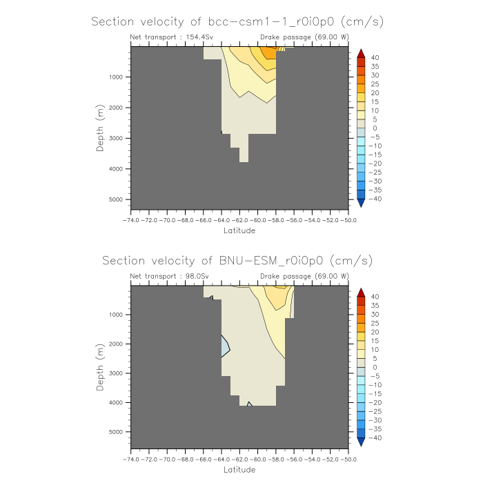
Recipe for russell et al figure 4. Plots the zonal velocity through Drake Passage (at 69W) and total transport through the passage if the volcello file is available.


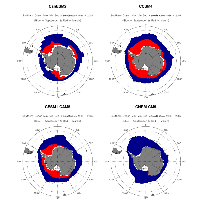
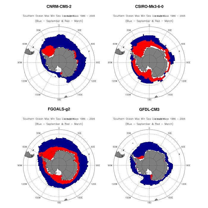
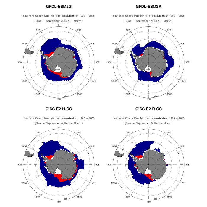
Diagnostic for russell et al figure 5 (polar). Plots the mean extent of sea ice for September(max) in blue and mean extent of sea ice for February(min) in red. The edge of full coverage is defined by the 15% areal coverage.

Recipe for russell et al figure 5g. Plots the annual cycle of sea ice area in southern ocean. The diag_script manually calculates the areacello for lat-lon models, as some models use different grids for areacello and sic files.
Diagnostic for russell et al Figure 6 (volume transport). Plots the density layer based volume transport(in Sv) across 30S based on the layer definitions in Talley (2008). The dark blue bars are the integrated totals for each layer and can be compared to the magenta lines, which are the observed values from Talley( 2008). The narrower red bars are equal subdivisions of each blue layer

Diagnostic for russell et al Figure 6b(heat transport). Plots the density layer based heat transport (in PW) across 30S based on the layer definitions in Talley (2008). The dark blue bars are the integrated totals for each layer and can be compared to the magenta lines, which are the observed values from Talley (2008). The narrower red bars are equal subdivisions of each blue layer

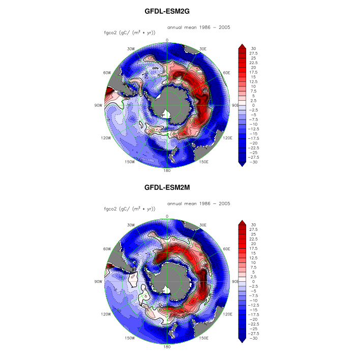
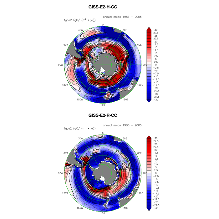
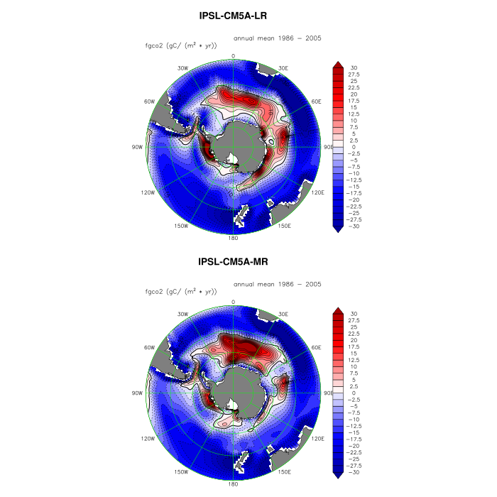
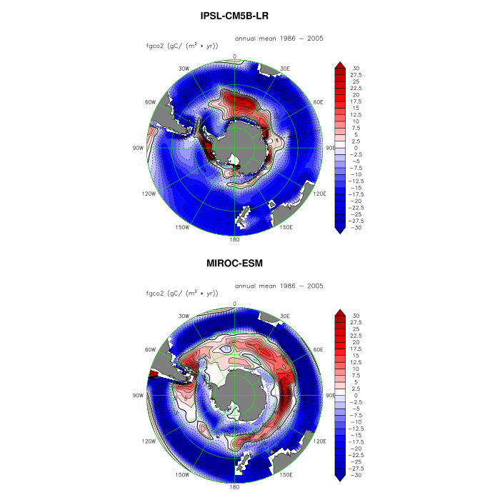
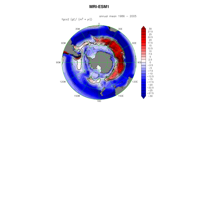
Diagnostic for russell et al figure 7(polar). Plots Annual mean CO2 flux (sea to air, gC/(yr * m^2), positive (red) is out of the ocean).

Diagnostic for russell et al figure 7h. Plots the zonal mean flux of fgco2 in gC/(yr * m^2).

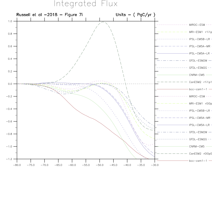
Diagnostic for russell et al figure 7i. Plots the cumulative integral of the net CO2 flux from 90S to 30S (in PgC/yr). The diag_script manually calculates the areacello for lat-lon models, as some models use different grids for areacello and fgco2 files.
Diagnostic for russell et al figure 8. Plots Surface pH in polar contour plot.


Diagnostic for russell et al figure 9a. Plots the scatter plot of the width of the Southern Hemisphere westerly wind band against the annual-mean integrated heat uptake south of 30S (in PW—negative uptake is heat lost from the ocean), along with the line of best fit. The diagnostic script will be updated later to include tauu variable and non-hfds datasets hfds = rsds + rlds - (rsus + rlus + hfss + hfls)

Diagnostic for russell et al figure 9b. Plots the scatter plot of the width of the Southern Hemisphere westerly wind band against the annual-mean integrated carbon uptake south of 30S(in Pg C/yr), along with the line of best fit. The diagnostic script will be updated later to include tauu variable.

Diagnostic for russell et al Figure 9c. Plots the scatter plot of the net heat uptake south of 30S(in PW) against the annual-mean integrated carbon uptake south of 30S(in Pg C/yr), along with the line of best fit. The diagnostic script will be updated later to include non-hfds datasets. hfds = rsds + rlds - (rsus + rlus + hfss + hfls)

main_log.txt | main_log_debug.txt | recipe_russell18jgr.yml | figures | data